This project wanted to look at associations between Willow Tit occurrence and environmental variables to see if any relationships were identified that could then be used as predictors of distribution in areas that were not sampled. Such an approach would potentially help identify sites that could be managed for Willow Tits.
However, it is worth noting that my knowledge of, and experience with, species distribution models is very limited. Therefore, I have relied heavily on Strimas-Mackey (2023) for guidance and recommendations in applying these methods to the data. As well, the following sections have been undertaken more as a means of teaching myself species distribution modeling using a case study, and so the results may not reflect a robust methodology for Willow Tit data analysis.
First, MODIS files were downloaded and processed into a raster file (see Processing_MODIS_files.R), then the variables were matched to the checklist locations and a prediction grid was created (see EnvironmentalVariables.R).
Landcover
The MODIS MCD12Q1 v061 product was the chosen dataset for landcover variables as it provides global coverage at 500m spacial resolution from 2001-present. The University of Maryland classification system was used. It provides fifteen classes:
| 0 |
Water bodies |
water |
At least 60% of area is covered by permanent water bodies. |
| 1 |
Evergreen Needleleaf Forests |
evergreen_needleleaf |
Dominated by evergreen conifer trees (canopy >2m). Tree cover >60%. |
| 2 |
Evergreen Broadleaf Forests |
evergreen_broadleaf |
Dominated by evergreen broadleaf and palmate trees (canopy >2m). Tree cover >60%. |
| 3 |
Deciduous Needleleaf Forests |
deciduous_needleleaf |
Dominated by deciduous needleleaf (e.g. larch) trees (canopy >2m). Tree cover >60%. |
| 4 |
Deciduous Broadleaf Forests |
deciduous_broadleaf |
Dominated by deciduous broadleaf trees (canopy >2m). Tree cover >60%. |
| 5 |
Mixed Forests |
mixed_forest |
Dominated by neither deciduous nor evergreen (40-60% of each) tree type (canopy >2m). Tree cover >60%. |
| 6 |
Closed Shrublands |
closed_shrubland |
Dominated by woody perennials (1-2m height) >60% cover. |
| 7 |
Open Shrublands |
open_shrubland |
Dominated by woody perennials (1-2m height) 10-60% cover. |
| 8 |
Woody Savannas |
woody_savanna |
Tree cover 30-60% (canopy >2m). |
| 9 |
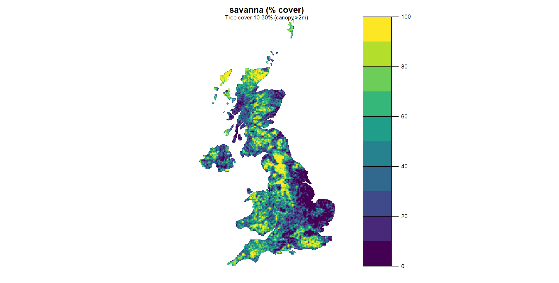
Savannas |
savanna |
Tree cover 10-30% (canopy >2m). |
| 10 |
Grasslands |
grassland |
Dominated by herbaceous annuals (<2m). |
| 12 |
Croplands |
cropland |
At least 60% of area is cultivated cropland. |
| 13 |
Urban and Built-up Lands |
urban |
At least 30% impervious surface area including building materials, asphalt, and vehicles. |
| 15 |
Non-Vegetated Lands |
nonvegetated |
At least 60% of area is non-vegetated barren (sand, rock, soil) or permanent snow and ice with less than 10% vegetation. |
| 255 |
Unclassified |
unclassified |
Has not received a map label because of missing inputs. |
University of Maryland classes
The landcover class was extracted for each checklist location by creating a 3km area around the checklist location. This is considered sufficient to account for spatial precision. Then, two metrics were calculated: a measure of composition (percentage of cover type) and a measure of configuration (edge density). These are reliable metrics for calculating environmental covariates in distribution models.
Elevation
Elevation data was downloaded from the EarthEnv website at 1km resolution. Then, both the mean and standard deviation of the elevation for the 3km checklist neighborhood was calculated.
The landcover and elevation variables were joined to the checklist data.
Prediction grid
A grid of habitat variables was created from which to make predictions.
The prediction grid was saved as a .csv file, but the raster (or .tiff) file can be used to map the variables. This is useful as a way to understand the classification scheme and how it relates to UK habitats.
For example, the variable “savanna” defined as “tree cover 30-60% (canopy >2m), was more relateable when mapped:
Example of mean elevation: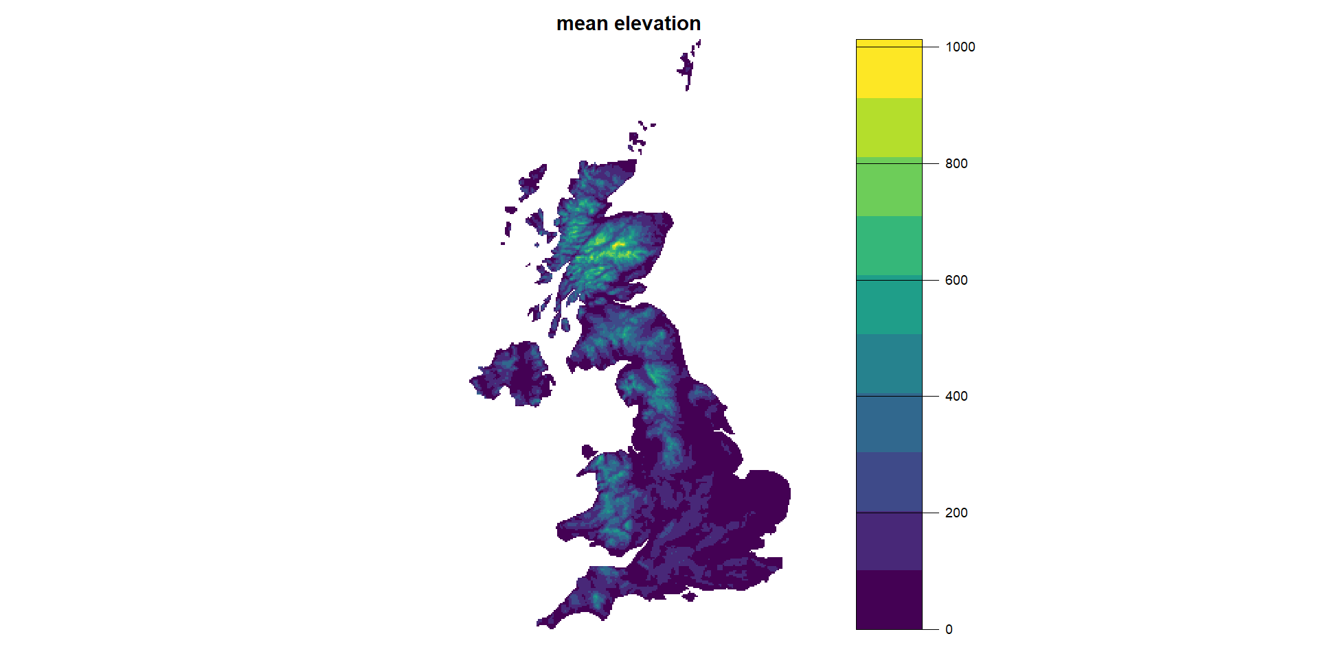
Strimas-Mackey, Hochachka, M. 2023.
“Best Practices for Using eBird Data.” Ithica, New York: Cornell Lab of Ornithology.
https://doi.org/10.5281/zenodo.3620739.